Strategic Aerospace Trends Radar

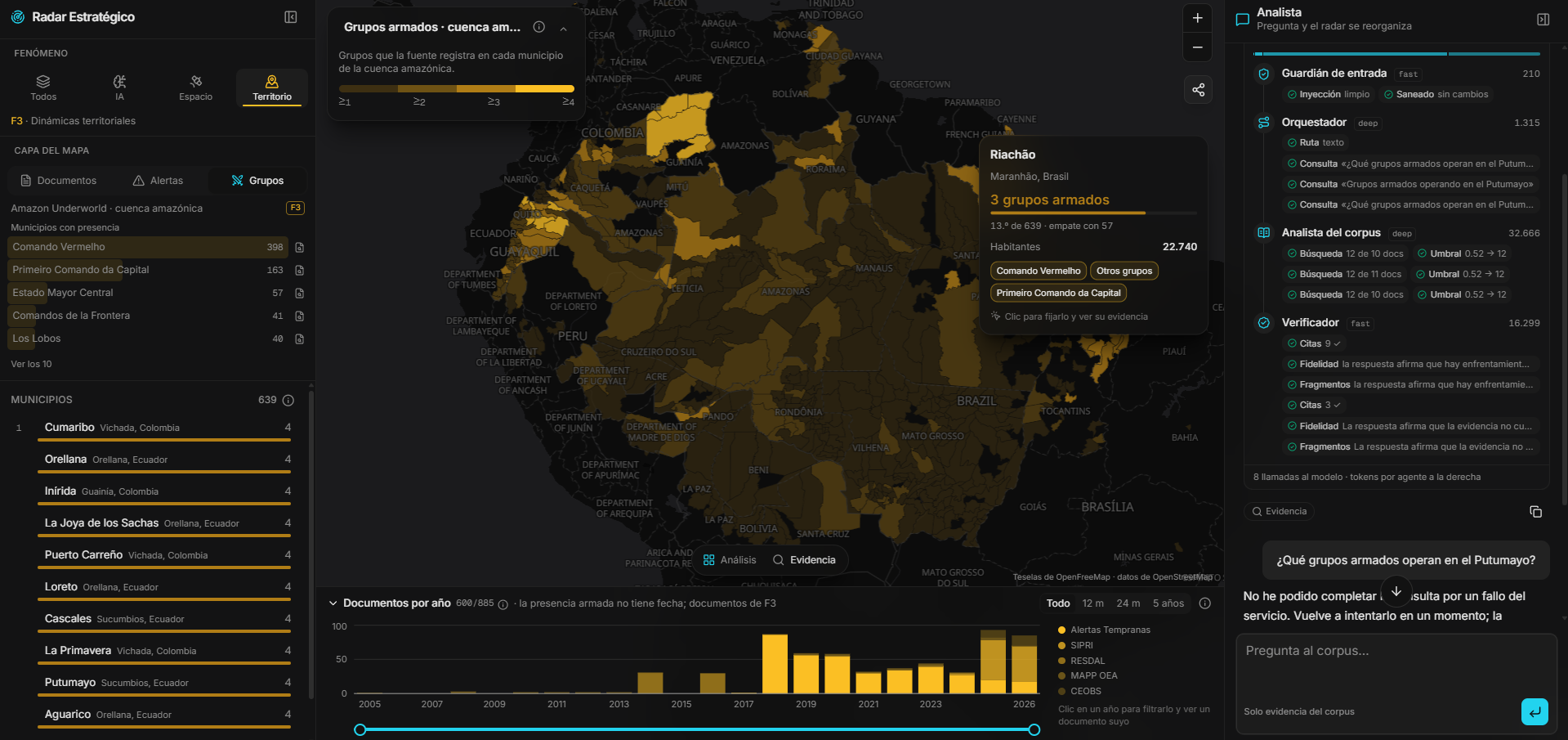
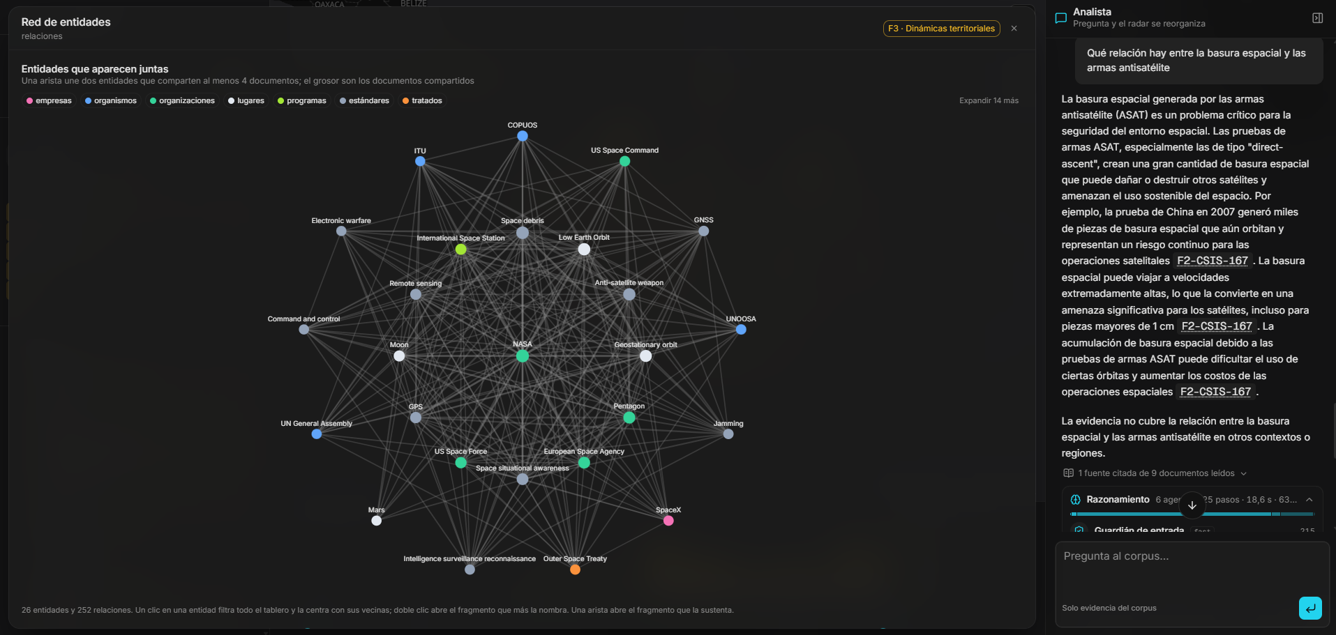
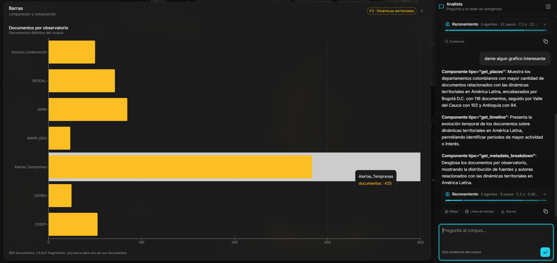
The Strategic Aerospace Trends Radar spares a security and defense analyst from reading thousands of documents by hand to understand three phenomena: artificial intelligence in military settings, the security of the space environment and low Earth orbit, and territorial dynamics in Latin America and the Caribbean. It answers natural-language questions, drives an interactive dashboard to show the answer, and traces every figure back to the exact passage it came from. We built it as team Aphelion at Codefest Ad Astra 2026, the hackathon run by the Colombian Aerospace Force and Universidad de los Andes, across two stages: first a multilingual knowledge base over the challenge corpus, then the multi-agent system and dashboard on top of it. We made it to the final.

The Challenge in Two Stages

The organizers handed every team the same corpus: 1,826 files about the three phenomena, from defense think tanks, space agencies, and Colombia's Ombudsman's Office. Each stage was graded separately, and the grading shaped almost every decision below.

• Stage 1 — the knowledge base. Answer 50 Spanish questions against a mostly English corpus with the top 3 documents and top 10 passages for each. Passages were scored by NDCG@10, documents by F1@3, in two independent leaderboards combined by Borda count. No generative model was allowed anywhere in indexing or retrieval.
• Stage 2 — the radar. Two challenges on top of that index. The assistant (POST /chat) was scored on answer quality (relevancy, faithfulness, toxicity, tone), efficiency (tokens, model calls, and latency, normalized against the other teams), security (75% of it by attacking the deployed endpoint with prompt injection), and design. The dashboard was scored mostly on dynamic execution: whether the agent activates the right component with the right data for each question.
• Hard rules for both: every visual claim traceable to its doc_id and chunk_id, no invented risk scores, no credentials in the code, and a budget of USD 100 in model spend. Once spent, the key stopped responding and there was no demo.

Stage 1: The Knowledge Base

Core Architecture

• Language: Python 3.12, a single self-contained generador.py that reproduces the submission from the persisted indexes
• Encoders: BAAI/bge-m3 and intfloat/multilingual-e5-large, both MIT-licensed XLM-RoBERTa encoders, loaded with sentence-transformers
• Index: FAISS IndexFlatIP on unit-normalized vectors, one per encoder, with a line-aligned metadata.jsonl
• Ingestion: PyMuPDF for PDFs, Tesseract OCR for scanned reports, and pysbd for sentence segmentation by detected language
• Evaluation: our own ground truth over the 50 real questions, with paired significance tests per question

Retrieval Pipeline

encode the question with each encoder (the same ones used at indexing time)
search each index for 200 candidates
passages:  BGE-M3 ranking → phenomenon boost → dedupe by text → max 3 per document → top 10
documents: convex fusion of both encoders → phenomenon boost → top-2 aggregation by source → top 3
validate the output format before writing it

The Corpus, Measured

We measured the corpus before designing anything. The 1,826 files split into 759 PDFs (131.6M characters of extracted text), 954 JSON files, 73 PBF map tiles, 26 CSVs (111.9M characters on their own), 6 XLSX workbooks, and a handful of images and text files. Four facts drove the design:

• 60 PDFs had no text layer. 48 of them were scanned Ombudsman reports that answer questions 33 to 50 directly, so OCR was mandatory.
• Language asymmetry. The 50 questions are in Spanish; 87% of the corpus is in English, with some Portuguese. Cross-lingual retrieval was the core problem, not an edge case.
• Extreme size spread. 1,300-character JSON alerts sit next to atlases hundreds of pages long.
• 59 file names repeat across 186 files with different content, verified by hash. That changes how documents must be counted for F1@3.

The final index holds 64,484 passages from 1,813 documents.

Chunking

Passages are built by accumulating complete sentences up to a token budget, so no sentence ever crosses a boundary, with a 15% overlap made of the previous passage's last whole sentences. Segmentation runs per document in its detected language; Portuguese is mapped to the English segmenter because pysbd rejects it, and without that mapping its 7,617 passages fell back to treating each paragraph as one sentence.

Two decisions came from measurement:

• A 400-passage cap per tabular file. 30 CSV/XLSX files produced 61% of the 149,571 initial passages, and three PubMed bibliography exports alone took 51.5%: biomedical references unrelated to any question, eating half the encoding time and competing in every search. Long legitimate PDFs are left untouched, and no file is excluded, because a document must stay reachable.
• Hierarchical chunking, tested and dropped. Splitting by detected headings scored NDCG@10 0.3602 against 0.4879 for sentence-bounded chunks on the same sample, the worst of every strategy we tried; heading detection is unreliable in a corpus with such mixed formatting.

Choosing the Encoders

Cross-lingual retrieval was the deciding criterion. BGE-M3 is trained explicitly for it (67.8 nDCG@10 on MIRACL across 18 languages, against 65.4 for mE5-large) and has an 8,192-token window; mE5-large has 512. Both are encoders, which the rules required: every model derived from an autoregressive backbone (Qwen3-Embedding, e5-mistral) was out regardless of its MTEB rank, and Jina v3 was out for its non-commercial license.

We compared seven encoders on a sample with our own ground truth. multilingual-e5-base fell far behind (NDCG@10 0.2503), gte-multilingual-base didn't beat the main pair despite adding a different pretraining family, and LaBSE, included as a control because it was trained to align parallel sentences rather than to judge relevance, confirmed the hypothesis by losing.

One configuration trap is worth recording: BGE-M3 pools the CLS token and mE5-large averages with the attention mask. Using mean pooling on BGE-M3 by mistake drops the cosine against the reference from 0.999999 to 0.81, an error that looks numeric but is a setting.

One Policy per Metric

Nothing in the rules forced passages and documents to come from the same ranking, and measured on the full corpus they shouldn't:

• BGE-M3 alone, top-2: NDCG@10 0.7329, F1@3 0.7000
• BGE-M3 + mE5-large, convex fusion, top-2: NDCG@10 0.6597, F1@3 0.7547
• BGE-M3 + mE5-large, RRF, top-2: NDCG@10 0.6255, F1@3 0.7413
• Adopted, passages from BGE-M3 and documents from convex fusion: NDCG@10 0.7329, F1@3 0.7547

Fusing the passages would cost 0.0732 NDCG@10 (p = 0.0012); not fusing the documents would cost 0.0547 F1@3. mE5-large brings in documents BGE-M3 misses, but it muddies the passage order. Convex fusion min-max normalizes each encoder per query before adding, because mE5-large compresses its similarities into 0.75–0.92 while BGE-M3 ranges lower, and unlike RRF it keeps the size of a win instead of reducing it to a position.

We were explicit about the limits: the F1@3 gain alone isn't significant (p = 0.1215). We kept it because against our own ground truth its cost is exactly zero, since the passage list doesn't change, and because the effect pointed the same way in every fusion variant we tried.

Ranking Rules, Each One Measured

• Phenomenon boost (×1.05), not a hard filter. Questions 5 and 46 treat Colombia from different phenomena, and question 27 crosses AI with space operations; a hard filter would drop valid evidence.
• Deduplication by text. 6.9% of the passages repeat one already indexed (reprinted tables, institutional headers). Two copies would spend two of ten slots saying the same thing. Duplicates are removed from the passage list, not from document aggregation, where dropping one could make a distinct document unreachable.
• At most 3 passages per document. Without the cap, one wrong document can take all ten slots and sink the question.
• Documents scored by top-2 and grouped by source. A document's score is the mean of its two best passages: summing favors long documents (forty passages at 0.15 add up to 6.0 and bury a short report with the exact answer at 0.85), and top-2 raised phenomenon 2's F1@3 from 0.7708 to 0.8750 over max. Grouping by source file rather than doc_id stops two copies of the same file from taking two of the three slots.

Results

Against our own ground truth: 1,383 graded passage judgments over 265 documents (relevance 0/1/2), pooled from the union of each encoder's top 15 so the measure isn't biased toward what the current configuration already finds.

• Overall (50 questions): NDCG@10 0.7329, F1@3 0.7547
• Phenomenon 1, AI in military settings: NDCG@10 0.6658, F1@3 0.6042
• Phenomenon 2, space security: NDCG@10 0.8382, F1@3 0.8958
• Phenomenon 3, territorial dynamics: NDCG@10 0.6988, F1@3 0.7630

Phenomenon 1 is the weakest on both metrics, and the corpus explains it: 6.4 relevant documents per question against 9.9 for phenomenon 2. There is less to find.

Measured and Discarded

• Pseudo-relevance feedback (Rocchio) over a 14-configuration grid: the best one moved NDCG@10 from 0.4879 to 0.5034 with p = 0.047, which doesn't survive correction for multiple comparisons, and it hurt F1@3 in all eight fusion settings. It stays implemented and disabled.
• Candidate pool depth: F1@3 rises steadily up to 200 candidates and flattens after (400 to 3,200 add nothing), so 200 is where it saturates, not an inherited number.
• Approximate indexes (IVF, HNSW): 64,484 vectors of 1,024 dimensions take about 252 MB per encoder and exhaustive search over 50 questions finishes in seconds. Stage 1 graded quality, not speed, so any lost recall would have been pure cost.
• The optional knowledge graph: we spent that time measuring the retrieval policy instead, which is what the stage graded.

Stage 2: The Multi-Agent Radar

Core Architecture

• Agent orchestration: LangGraph, with six agents in a graph with conditional routing and a capped verification loop
• Backend: FastAPI + asyncpg; a single process serves the challenge's POST /chat endpoint, an SSE stream, and the dashboard's aggregation API
• Models: gpt-oss-120b to route, decompose, and write, and gpt-oss-20b for the guards, the visualizer, and the verifier, through an OpenAI-compatible LiteLLM proxy
• Retrieval: the Stage 1 BGE-M3 vectors moved into PostgreSQL 18 + pgvector behind an HNSW index, so a single query crosses vectors and metadata without leaving the database
• Frontend: Next.js 16 + TypeScript + MapLibre + Recharts + AI Elements; the same image serves the dashboard and the chat depending on NEXT_PUBLIC_SURFACE
• Contract: Pydantic response models, with the frontend's types generated from the backend's OpenAPI
• Deployment: three Coolify resources built from Dockerfiles, with non-root images and a HEALTHCHECK

Layered Architecture

The dashboard and the chat are two deployments of the same frontend image, backed by a single backend. The agent's tools and the dashboard's components query exactly the same aggregation endpoints, so a figure can't say one thing in the chat and another on the map. Splitting them would have meant maintaining the same aggregation twice and risking that they drift apart. They are two separate deployments on purpose: the assistant was evaluated in a closed window, and redeploying the dashboard couldn't be allowed to take the chat down.

Request Flow

Agent Graph

Six agents in a LangGraph graph. Three are the minimum the challenge required; the other three handle security and verification, because attack resistance was graded by attacking the deployed system. Every early exit (an attack, a greeting, a question with no evidence) ends the run without spending calls it no longer needs.

• input_guardrail (small model): classifies the message before it enters the graph, so a direct attack is cut before the large model is paid for.
• orchestrator (large model): picks the route and breaks the question into search formulations, in one call.
• rag_analyst (large model): retrieves and writes with the evidence; this is the system's actual reasoning.
• visualizer (small model): picks the dashboard components that answer the question and their filters. Choosing what to look at isn't writing, so only the questions that need it pay for it.
• verifier (small model): checks faithfulness, traceability, and indirect injection. Auditing is easier than writing.
• output_guardrail (small model): toxicity and leaked instructions, the last barrier on text a model already wrote.

When the verifier rejects an answer, the orchestrator reformulates with the reason in front of it and the analyst retrieves and writes again, at most twice. Past that cap the answer ships with the status no_verificada, declared rather than failing.

Three Routes, Decided in One Call

• text: only the analyst runs, for explanations, doctrine, causes, and context.
• visualization: only the visualizer runs, for a figure spread over space, time, or categories. This route skips the verifier, because there are no retrieved passages whose citations it could check; the output guard still runs.
• both: the two branches run in parallel and meet again at the writer, so choosing the components adds no wall-clock latency.

On any failure the route falls back to text, which is what the system already did. If the visual route produces no valid component, the answer still comes from the corpus and says that the visualization couldn't be prepared.

Security in Layers

Direct attacks are mostly stopped by the model's own alignment. The one that actually gets through is indirect: an instruction riding inside a retrieved passage, because the corpus holds documents nobody wrote with an assistant in mind. Each layer covers what the previous one can't:

• Input classifier: instruction overrides, system-prompt extraction, impersonation, jailbreaks.
• Retrieved context fenced and declared as data: the defense that actually stops indirect injection.
• A writer with no tools: a poisoned passage has no action to invoke.
• Citation check in code: invented references, which a prompt can't prevent.
• Output classifier: toxicity and leaks of the system prompt.
• A hard iteration cap: budget exhaustion.
• Credentials only through environment variables: no secret in the repository or the image, which the static analysis checked.

A Response Contract That Can't Drift

The response models follow the challenge's specification field by field, all with extra="forbid", and the response is assembled in one place from the graph's final state whichever path it took, so no path can return a field too many or too few. Tokens are accumulated per agent rather than per model (two agents share a model), num_interacciones counts model calls, and latency is measured around the graph run. Every failure still returns the full contract with its status, never a bare 500: during the evaluation window a failed request was a lost question with no retry. An internal error is never reported as sin_evidencia, because saying the corpus has no evidence when the proxy is what went down would be a false claim about the corpus.

Key Features

Tools at a Glance

The assistant drives the dashboard

A question that asks to see something (where, when, with whom, what dominates) goes through the visualizer agent, which doesn't write: it picks one to three components and their filters. It never picks the data, which comes from the same aggregation endpoints that draw the dashboard, and everything it returns is validated in code against closed lists, so a tool, field, or entity that doesn't exist is dropped. The component is inferred from the tool name, which already travels in the agent's response, so coordinating the dashboard costs zero extra tokens and adding a component means adding a tool. If the question names a territory, the code resolves it against the places table, and the map frames it and opens its evidence as if it had been clicked.

A component for each analytical task

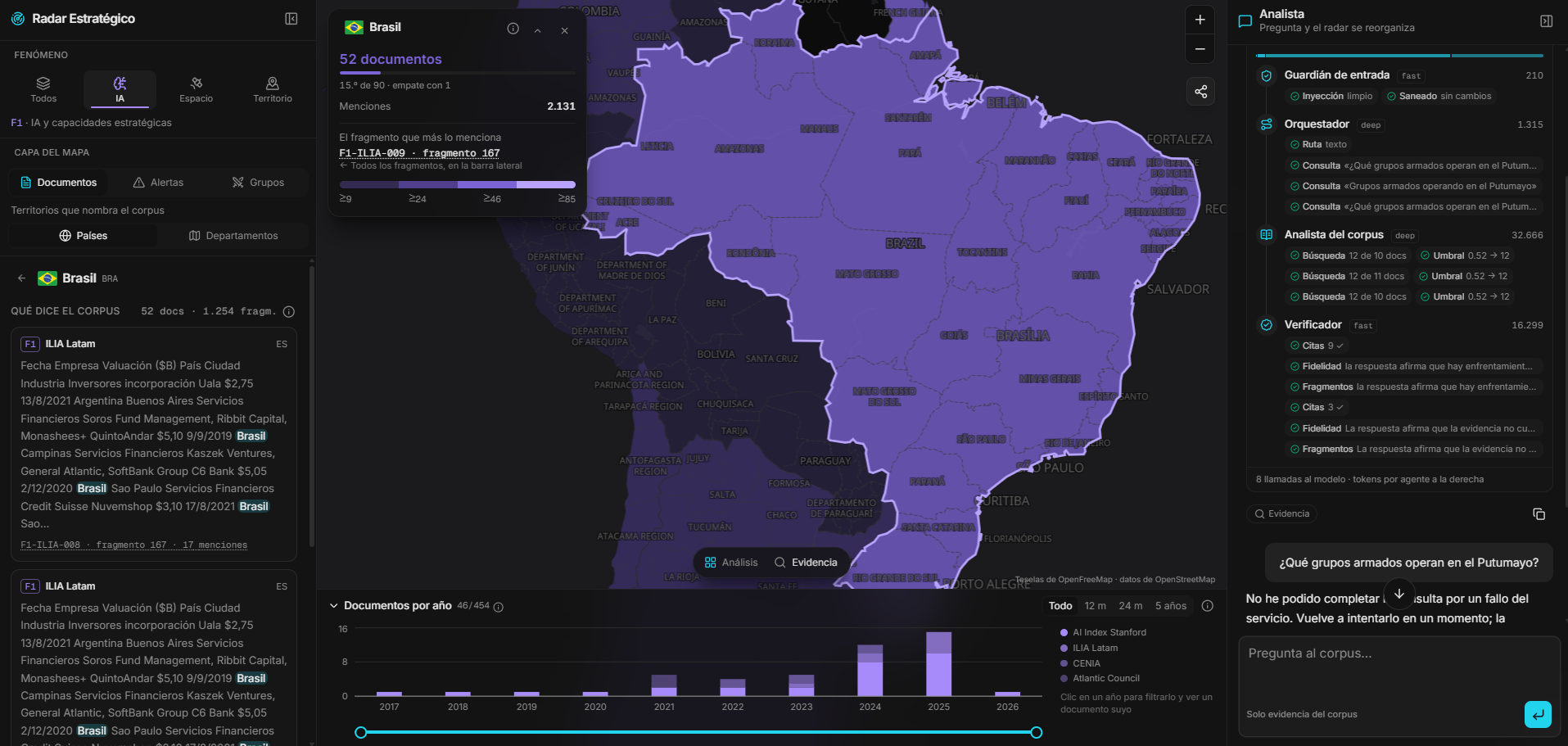
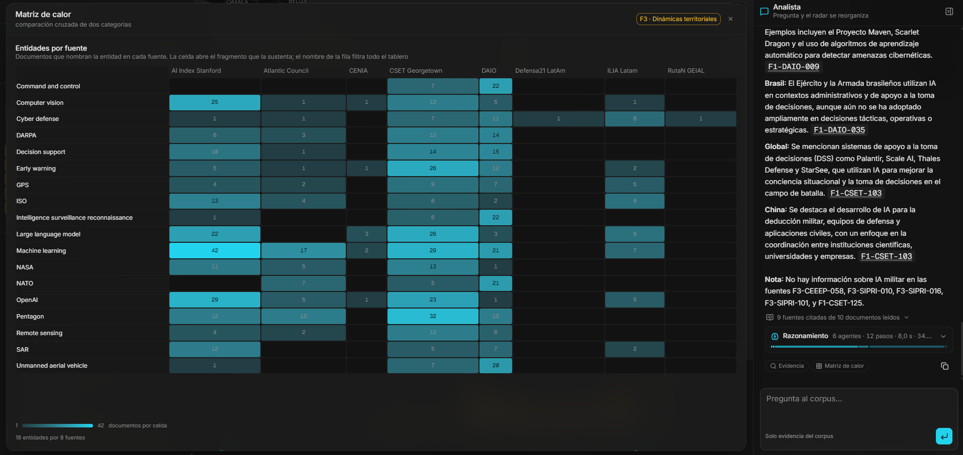
The components were chosen backwards from the usual order: first the questions each phenomenon makes it reasonable to ask, then the chart that answers them. Comparisons get bars, cross-comparisons a heat matrix, relationships a co-occurrence network, spatial distribution a choropleth, trends a timeline, and verification the evidence panel.

• AI in military settings is about actors and programs, not territory, so its main views are the heat matrix and the co-occurrence network.
• Space security is about an agenda: which concerns are growing and which have settled. Its main view is an intensity-versus-trend quadrant, with the timeline.
• Territorial dynamics is the only phenomenon with an explicit territory, so the choropleth leads, with the network and the evidence panel alongside.

One map, three different questions

The map doesn't stack layers: each view is a different question about a different territory, and mixing them would produce a color that means nothing.

• Documents: how many corpus documents name each country or department. Naming isn't acting.
• Alerts: which departments the Ombudsman's 363 early warnings (2017–2026) name, split into imminent and structural risk, never added together.
• Armed groups: which groups are present in each of 1,407 municipalities across six Amazon countries, from the public Amazon Underworld dataset. It's declared presence, not intensity, and a municipality without information is never shown as one without presence.

Armed presence is drawn municipality by municipality because that's the level the source measures: aggregating to the department would erase the difference between a municipality with four groups and one with none. The municipal shapes didn't survive Stage 1 indexing, so they come from geoBoundaries and are matched by name, with repeated names resolved by which department contains the polygon's center: 1,385 of the 1,407 municipalities (98%) find their shape.

No number without a source

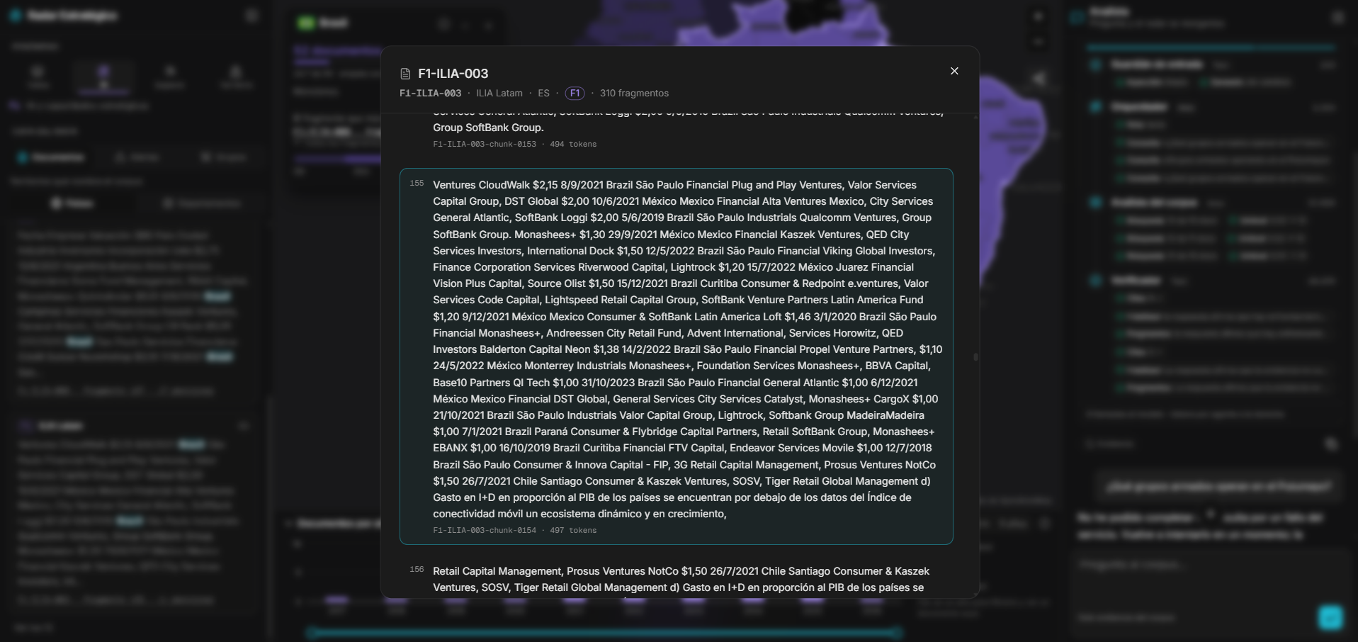
Every bar, cell, year, node, or territory on the dashboard carries the doc_id and chunk_id of a passage that its figure counts. One click opens the document at that passage, with every mention highlighted using the exact forms the precompute counted. The document view serves an 80-passage window centered on the citation rather than the whole document; the largest has 1,960 passages. The system counts and aggregates, but never computes a risk score of its own: the rules forbade it, and a number without a source is useless to someone who has to decide with it.

Filters that live in the URL

The phenomenon, the period, and the selected entity carry across every view and live in the URL, so any view can be shared exactly as it is and the back button works. Selecting an entity in the matrix, the network, or the quadrant narrows the other views to the documents that name it. The period filter is monthly, but only 212 documents carry a full date, so a document enters only when its whole known date falls inside the period. The share button composes an image card of the view (map, filters, legend, ranking, and source) instead of a raw screenshot.

Visible reasoning

Every answer shows its linked citations, the sources it read, and its reasoning: which agents took part, in what order, with which model, how many tokens they spent, and what each tool returned. While the graph runs, the frontend receives each node over SSE as soon as it finishes.

Technical Highlights

The writer has no tools

Retrieving and writing are two separate nodes. The one that writes takes text and returns text, so a poisoned passage has nothing to invoke even if it fools the model. It's the only defense that stops indirect injection by construction. For the same reason the model doesn't decide whether to search: every question about the content needs evidence, so asking would be paying a call for an answer already known.

Traceability is checked in code

Knowing whether a cited identifier is among the retrieved passages is a set comparison: exact, free, and infallible, so no model is asked. A measured lesson: gpt-oss-120b writes citations with the non-breaking hyphen (U+2011) and spaces inside the brackets. With the naive pattern no citation was extracted, and the answer passed verification without anyone having looked at its sources, which is worse than having no check at all. Hyphens and spaces are now normalized before extraction.

A budget in dollars, not tokens

With USD 100 for the whole event, everything that isn't reasoning goes to the small model, every call uses reasoning_effort: "low" (on a simple "say hello", 23 of 33 output tokens were reasoning), and greetings or off-topic questions are answered without walking the graph. max_tokens is never tightened: these models reason before answering, and with a tight margin they spend the budget reasoning and emit nothing. Measured end to end: a full question is 6 model calls, about 33,000 tokens, and 17 s; an attack dies at the first layer with 1 call, 344 tokens, and 1.2 s.

Routing costs no extra calls

The orchestrator picks the route in the same call it uses to decompose the question, as one more field in the JSON it already returned. The text route therefore costs exactly what it did before the visualizer existed, which mattered because efficiency was scored against the other teams.

The guards fail open, and stay quiet

If the model proxy doesn't respond, the guards let the message through instead of blocking: turning a provider outage into a blanket block would take the demo down, and the other layers still stand. When an input is blocked, the response doesn't say which rule fired, so the attacker isn't taught their next attempt; the reason stays in the structured log.

Structured data recovered from the index

The alerts and armed-presence layers were rebuilt from the index itself, without going back to the raw corpus: those documents kept their structured fields inside the indexed text (b_ADM2_PCODE, au_eln, fecha_emision), so the data was in the database in the form of sentences. Entities are extracted by dictionary and text matching rather than an LLM: running 1,813 documents through inference would have eaten the budget, and proper names don't need reasoning.

Dates from the source, never from the text

A year mentioned inside a report is the year it talks about, not the year it was published, so publication dates come only from source metadata: the file name and its folder in the original corpus. Five rules, from most to least precise (alert number, year in the name, ISO date, year folder, compact date), and every row records which rule produced it, so any point on the timeline can be audited back to its file. 965 of 1,813 documents get a date; the rest stay out of the series, and the timeline says so in its own header instead of spreading them around.

Trend without inventing a score

The intensity-versus-trend quadrant uses only verifiable counts: how many dated documents name the entity, and what share of them sits in the recent half of the corpus. The cutoff is the median of the dated corpus, computed rather than fixed, and the dividing lines are each axis's median, so the quadrant compares entities with each other rather than against an invented threshold.

A data audit before delivery

Place counts were audited against the text. Natural Earth gives Bogotá the code for Cundinamarca, so every mention of the capital counted for the department; Bogotá now has its own code. Homonyms (an armed group named after a department, a treaty, a university) were added as decoys, which dropped Santander from 59 to 41 documents. And the Ombudsman's postal addresses, printed on every alert and spelled differently by OCR each time, are stripped before searching.

Project Structure

Stage 1, the knowledge base submission:

generador.py          # self-contained: reproduces resultados.jsonl from the persisted indexes
resultados.jsonl      # 50 lines, 3 documents and 10 passages per question
base_vectorial/
├── encoder_bge-m3/     # index.faiss + metadata.jsonl, line n describes vector n
└── encoder_me5-large/  # the same for multilingual-E5-large
informe_tecnico.pdf   # technical report: design, measurements, and each decision's rationale
requirements.txt      # pinned versions, verified in a clean environment

Stage 2, the radar:

backend/
├── app/
│   ├── agent/        # LangGraph graph: guards, orchestrator, analyst, visualizer, verifier
│   ├── api/          # POST /chat, the SSE stream, and the dashboard's aggregation endpoints
│   ├── db/           # per-component queries (places, timeline, entities, quadrant…)
│   └── responses.py  # the challenge's response contract, validated with extra="forbid"
├── precompute/       # entities, places, dates, armed presence, alerts, and municipalities, computed once
├── scripts/          # generates agent_card.json from the agent declarations
└── tests/            # guards, verifier, routing, and the full graph end to end with mocks
frontend/
├── app/              # Next.js 16 App Router
├── components/       # map, analysis components, chat, timeline, and the component registry
└── lib/              # API client with types generated from OpenAPI, filters, and URL state
docs/arquitectura.md  # the system design and the reasoning behind each decision

Impact and Scalability

• Finalist at Codefest Ad Astra 2026, with Stage 2 built and deployed in 24 hours of on-site development.
• One index, two stages: the vectors built and measured in Stage 1 are the ones the Stage 2 agents query, so the retrieval quality was settled before a single prompt was written.
• Reproducible by design: Stage 1's generator runs from its own folder with fixed seeds and pinned versions, and an automated test compares it against the development implementation so the two can't drift silently.
• Adding a component means adding a tool and its registry entry: the frontend infers it from the tool name.
• Switching model providers is four environment variables, not code: the challenge gateway and a development one speak the same dialect.
• Frontend types are generated from OpenAPI, so a backend response change is never written twice.
• Tests cover the guards with known injection cases, the verifier, and the full graph end to end with the proxy and the index mocked.

Notes

Built with Python, FAISS, LangGraph, FastAPI, PostgreSQL + pgvector, and Next.js. The code for both stages is public: Stage 1 (the knowledge base and its technical report) and Stage 2 (the agents and the dashboard). The organizers provided the corpus for the event only, so this page shows the solution, not the data.